相机模型总结

相机模型

相机模型就是用数学的方式描述了一个真实世界中的三维点到图像上像素坐标的映射关系。

前言

成像既然是用来描述真实的相机镜头的投影关系，那么必然理论跟现实就会有差距。因此，研究者设计了不同的成像模型来描述不同镜头的投影关系。也可以根据这些数学模型设计真实的物理镜头。事实上，只要成像角度稍微大的镜头（可以想象鱼眼镜头），如果还是用简单的针孔模型来描述的化，偏差就会很大，因此需要不同的相机模型来描述。

经典的成像模型要有一个步骤就是把三维坐标的点先投影到单位球(Unit Sphere)上，有时候这个单位球也叫Viewing Sphere

之所以可以这样做的原因是，从相机光心发射出的一条线，线上的点都会投影到同一个像素值。也就是说，我们在做投影的时候，放缩一个常量的结果是相同的

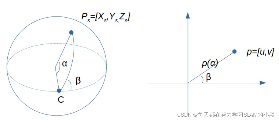
先把三维点投影到单位球上，其在图像上的成像点与图像y轴的夹角保持不变，其在图像上离原点的距离是夹角 α \alpha α的函数

P s = P ∥ P ∥ = ( x s , y s , z s ) r = x s 2 + y s 2 α = a t a n ( r , z s ) β = a t a n ( y s , x s ) P_{s}=\frac{P}{\|P\|}=\left(x_{s}, y_{s}, z_{s}\right) \\ r = \sqrt{x_s^2+y_s^2} \\ \alpha = atan(r,z_s) \\ \beta = atan(y_s,x_s) Ps​=∥P∥P​=(xs​,ys​,zs​)r=xs2​+ys2​ ​α=atan(r,zs​)β=atan(ys​,xs​)

是三维点投影到单位圆之后的点，该点投影到图像上，与图像x轴的夹角保持不变，其到图像中心的距离是夹角 的函数 ，这个函数的不同形式对应着不同的经典成像模型

1. pinhole 针孔模型

针孔相机有四个参数： f x , f y , c x , c y f_x,f_y,c_x,c_y fx​,fy​,cx​,cy​,投影方程定义为： π ( x , i ) = [ u v ] = [ f x x z f y y z ] + [ c x c y ] \boldsymbol{\pi}(\mathbf{x}, \mathbf{i})=\left[\begin{array}{l}u \\ v \end{array}\right]=\left[\begin{array}{l}f_{x} \frac{x}{z} \\ f_{y} \frac{y}{z}\end{array}\right]+\left[\begin{array}{l}c_{x} \\ c_{y}\end{array}\right] π(x,i)=[uv​]=[fx​zx​fy​zy​​]+[cx​cy​​]
或者 [ u v 1 ] = [ f x 0 c x 0 f y c y 0 0 1 ] [ X Z Y Z 1 ] \left[\begin{array}{l}u \\ v \\ 1\end{array}\right]=\left[\begin{array}{ccc}f_{x} & 0 & c_{x} \\ 0 & f_{y} & c_{y} \\ 0 & 0 & 1\end{array}\right]\left[\begin{array}{c}\frac{X}{Z} \\ \frac{Y}{Z} \\ 1\end{array}\right] ⎣⎡​uv1​⎦⎤​=⎣⎡​fx​00​0fy​0​cx​cy​1​⎦⎤​⎣⎡​ZX​ZY​1​⎦⎤​

代码实现

// cam2world（unprojection）
	if(!distortion_)
	  {
  
	    xyz[0] = (u - cx_)/fx_;
	    xyz[1] = (v - cy_)/fy_;
	    xyz[2] = 1.0;
	  }
	
// world2cam（projection）
	  if(!distortion_)
	  {
  
	    px[0] = fx_*uv[0] + cx_;
	    px[1] = fy_*uv[1] + cy_;
	  }

2. Omnidirectional Camera Model 全向相机模型

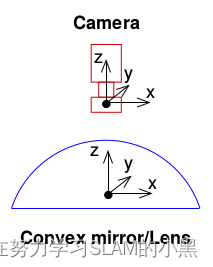
全向相机采用的镜片通常为凸透镜，所以感光传感器上汇聚的环境光会发生折射，导致坐标系点产生变化，如下图所示。将凸透镜片称为mirror系。由于有mirror系的存在，所以全向相机模型会比针孔相机模型多一个参数
全向相机（Omnidirectional Camera）模型有五个参数： ξ , f x , f y , c x , c y \xi, f_x,f_y,c_x,c_y ξ,fx​,fy​,cx​,cy​

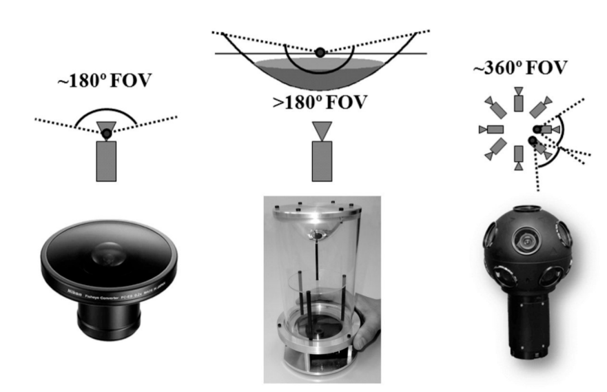
模型主要分为两种：

1. central cameras 有中心相机
2. non-central cameras 无中心相机
   
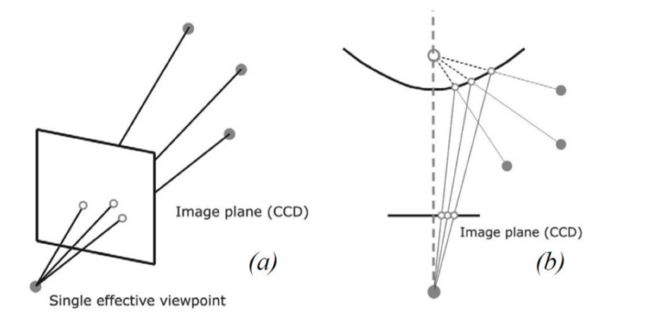
   这两种光都集中在中间一个点
   
   成像中心不是在一个点上
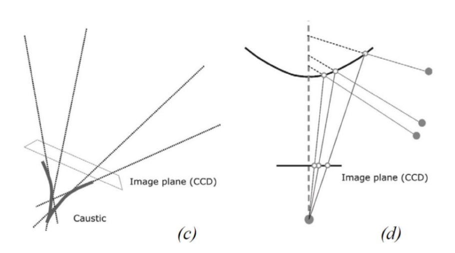
   (a，b)central cameras的例子:透视投影和双曲镜折射率投影。(c，d)non-central cameras 的例子:光线的包络形成焦散。

• 后面的模型主要是（b）

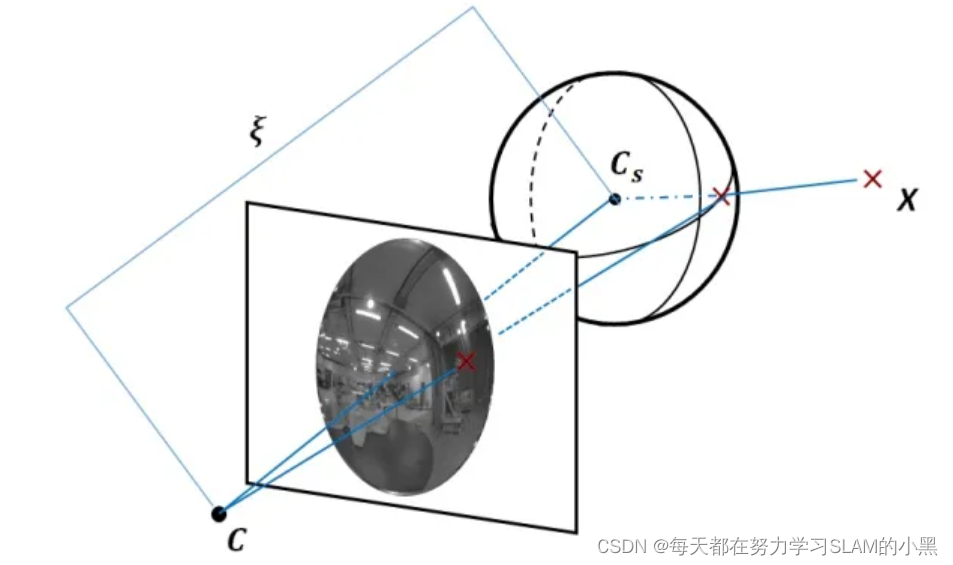
2.1 Unified model for catadioptric cameras 反射式相机统一模型

• 主要应用于反射式镜头，也可应用于鱼眼

• 我们构建模型的主要目标是获得 入射方向 和 像素坐标 的映射关系，针对相机坐标系下一个点 P = ( x , y , z ) P=(x,y,z) P=(x,y,z) (在相机坐标系下)， 其成像中心为 C C C

• 假设： 成像轴和镜面的反射轴是完美重合的

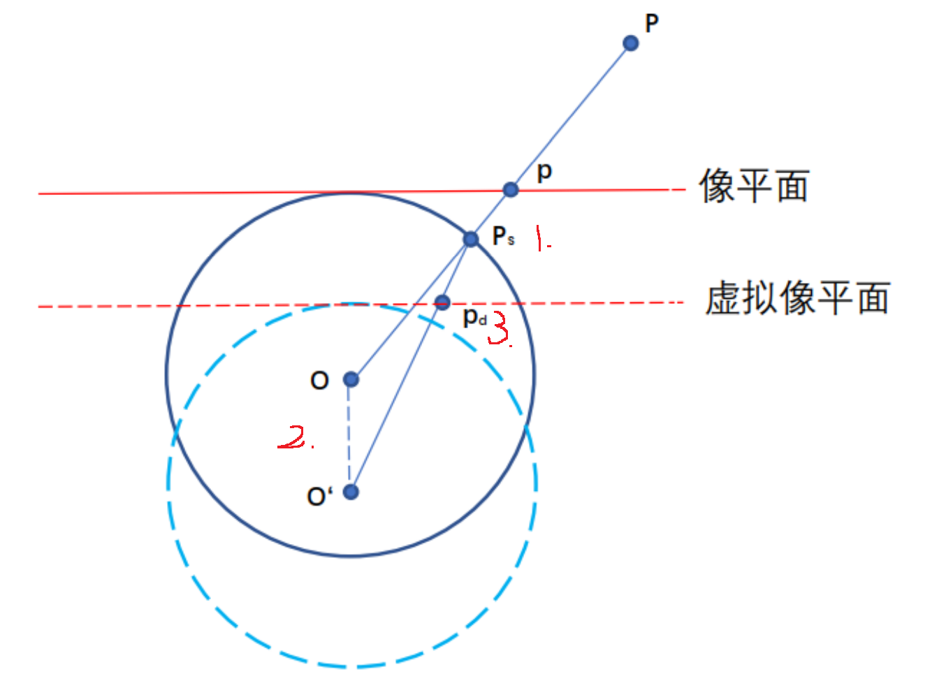
统一化的相机模型主要遵循以下几个步骤：

1. 将点 P P P 归一化到一个单位球上 （ ∣ ∣ P s ∣ ∣ = 1 ||P_{s}||=1 ∣∣Ps​∣∣=1）
   P s = P ∥ P ∥ = ( x s , y s , z s ) P_{s}=\frac{P}{\|P\|}=\left(x_{s}, y_{s}, z_{s}\right) Ps​=∥P∥P​=(xs​,ys​,zs​)
2. 将成像中心沿光轴调整到新的位置 C ξ = ( 0 , 0 , − ξ ) C_{\xi}=(0,0,-\xi) Cξ​=(0,0,−ξ), 有
   P ξ = ( x s , y s , z s + ξ ) P_{\xi}=\left(x_{s}, y_{s}, z_{s}+\xi\right) Pξ​=(xs​,ys​,zs​+ξ)
   

由于我们单位球，因此 ξ ∈ [ 0 , 1 ] \xi \in[0,1] ξ∈[0,1], 当其为 0 时，实际上就是我们的针孔模型。
3. 按照小孔成像的方式， 将点 P ξ P_{\xi} Pξ​ 投影至归一化成像平面
p d = ( x d , y d , 1 ) = ( x s z s + ξ , y s z s + ξ , 1 ) = g − 1 ( P ) p_{d}=\left(x_{d}, y_{d}, 1\right)=\left(\frac{x_{s}}{z_{s}+\xi}, \frac{y_{s}}{z_{s}+\xi}, 1\right)=g^{-1}(P) pd​=(xd​,yd​,1)=(zs​+ξxs​​,zs​+ξys​​,1)=g−1(P)

类比针孔相机,就是 ( x s z s , y s z s , 1 ) \left(\frac{x_{s}}{z_{s}}, \frac{y_{s}}{z_{s}}, 1\right) (zs​xs​​,zs​ys​​,1)

1. 按照小孔成像模式增加畸变项
   各种畸变模型，参考第二章
2. 使用内参矩阵 K K K 进行投影, 内参矩阵和第二章定义类似
   p = [ u v 1 ] = K p d p= \begin{bmatrix} u\\v\\1\end{bmatrix}=K p_{d} p=⎣⎡​uv1​⎦⎤​=Kpd​
   

反投影

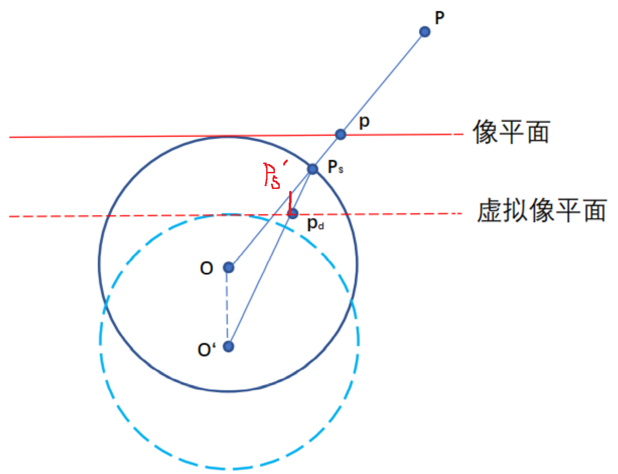
反投影实际上就是已知 p d p_{d} pd​ (归一化的图像坐标系的点)求解 P s P_{s} Ps​ 的过程，我们假设 O P s O P_{s} OPs​ 射线上存在一个点 P s ′ = ( x d , y d , z ′ ) P_{s}^{\prime}=\left(x_{d}, y_{d}, z^{\prime}\right) Ps′​=(xd​,yd​,z′) ，（其模长 = r 2 + z ′ 2 \sqrt{r^2+z'^2} r2+z′2 ​）其归一化后实际上就是 P s P_{s} Ps​, 也就是说，其成像点也是 P d P_{d} Pd​, 即其满足
( x d z ′ + ξ z ′ 2 + r 2 , y d z ′ + ξ z ′ 2 + r 2 , 1 ) = ( x d , y d , 1 ) \left(\frac{x_{d}}{z^{\prime}+\xi \sqrt{z^{\prime 2}+r^{2}}}, \frac{y_{d}}{z^{\prime}+\xi \sqrt{z^{\prime 2}+r^{2}}}, 1\right)=\left(x_{d}, y_{d}, 1\right) (z′+ξz′2+r2 ​xd​​,z′+ξz′2+r2 ​yd​​,1)=(xd​,yd​,1)

归一化时 = > ( x d z ′ 2 + r 2 , y d z ′ 2 + r 2 , z d z ′ 2 + r 2 ) => \left(\frac{x_{d}}{ \sqrt{z^{\prime 2}+r^{2}}}, \frac{y_{d}}{ \sqrt{z^{\prime 2}+r^{2}}}, \frac{z_{d}}{ \sqrt{z^{\prime 2}+r^{2}}}\right) =>(z′2+r2 ​xd​​,z′2+r2 ​yd​​,z′2+r2 ​zd​​)
= > ( x d z ′ 2 + r 2 ∗ ( z d z ′ 2 + r 2 + ξ ) + , y d z ′ 2 + r 2 ∗ ( z d z ′ 2 + r 2 + ξ ) , 1 ) =>\left(\frac{x_{d}}{ \sqrt{z^{\prime 2}+r^{2}}*(\frac{z_{d}}{ \sqrt{z^{\prime 2}+r^{2}}}+\xi)}+, \frac{y_{d}}{ \sqrt{z^{\prime 2}+r^{2}}*(\frac{z_{d}}{ \sqrt{z^{\prime 2}+r^{2}}}+\xi)}, 1\right) =>(z′2+r2 ​∗(z′2+r2 ​zd​​+ξ)xd​​+,z′2+r2 ​∗(z′2+r2 ​zd​​+ξ)yd​​,1)
= > ( x d z ′ + ξ z ′ 2 + r 2 , y d z ′ + ξ z ′ 2 + r 2 , 1 ) = ( x d , y d , 1 ) =>\left(\frac{x_{d}}{z^{\prime}+\xi \sqrt{z^{\prime 2}+r^{2}}}, \frac{y_{d}}{z^{\prime}+\xi \sqrt{z^{\prime 2}+r^{2}}}, 1\right)=\left(x_{d}, y_{d}, 1\right) =>(z′+ξz′2+r2 ​xd​​,z′+ξz′2+r2 ​yd​​,1)=(xd​,yd​,1)

则有
z ′ + ξ z ′ 2 + r 2 = 1 z^{\prime}+\xi \sqrt{z^{\prime 2}+r^{2}}=1 z′+ξz′2+r2 ​=1
因此有
z ′ = ξ 1 + r 2 ( 1 − ξ 2 ) − 1 ξ 2 − 1 z^{\prime}=\frac{\xi \sqrt{1+r^{2}\left(1-\xi^{2}\right)}-1}{\xi^{2}-1} z′=ξ2−1ξ1+r2(1−ξ2) ​−1​
我们稍微整理下，可以把上述的投影流程表达为(opencv形式)( γ x , c x , γ y , c y \gamma_{x},c_{x},\gamma_{y},c_{y} γx​,cx​,γy​,cy​相当于内参K)
π ( x , i ) = [ γ x x ξ d + z γ y y ξ d + z ] + [ c x c y ] d = x 2 + y 2 + z 2 \begin{aligned} \pi(\mathbf{x}, \mathbf{i}) &=\left[\begin{array}{l} \gamma_{x} \frac{x}{\xi d+z} \\ \gamma_{y} \frac{y}{\xi d+z} \end{array}\right]+\left[\begin{array}{l} c_{x} \\ c_{y} \end{array}\right] \\ d &=\sqrt{x^{2}+y^{2}+z^{2}} \end{aligned} π(x,i)d​=[γx​ξd+zx​γy​ξd+zy​​]+[cx​cy​​]=x2+y2+z2 ​​
实际上，我们会使用如下形式(kalibr形式)
π ( x , i ) = [ f x x α d + ( 1 − α ) z f y d α d + ( 1 − α ) z ] + [ c x c y ] \pi(\mathbf{x}, \mathbf{i})=\left[\begin{array}{c} f_{x} \frac{x}{\alpha d+(1-\alpha) z} \\ f_{y} \frac{d}{\alpha d+(1-\alpha) z} \end{array}\right]+\left[\begin{array}{c} c_x\\ c_y \end{array}\right] π(x,i)=[fx​αd+(1−α)zx​fy​αd+(1−α)zd​​]+[cx​cy​​]

其反投影为(kalibr形式，自行推导)
π − 1 ( u , i ) = ξ + 1 + ( 1 − ξ 2 ) r 2 1 + r 2 [ m x m y 1 ] − [ 0 0 ξ ] m x = v − c y f y ( 1 − α ) r 2 = m x 2 + m y 2 ξ = α 1 − α γ x = f x 1 − α γ y = f y 1 − α \begin{aligned} \pi^{-1}(\mathbf{u}, \mathbf{i}) &=\frac{\xi+\sqrt{1+\left(1-\xi^{2}\right) r^{2}}}{1+r^{2}}\left[\begin{array}{c} m_{x} \\ m_{y} \\ 1 \end{array}\right]-\left[\begin{array}{l} 0 \\ 0 \\ \xi \end{array}\right] \\ m_{x} &=\frac{v-c_{y}}{f_{y}}(1-\alpha) \\ r^{2} &=m_{x}^{2}+m_{y}^{2} \\ \xi &=\frac{\alpha}{1-\alpha} \\ \gamma_{x} &=\frac{f_{x}}{1-\alpha} \\ \gamma_{y} &=\frac{f_{y}}{1-\alpha} \end{aligned} π−1(u,i)mx​r2ξγx​γy​​=1+r2ξ+1+(1−ξ2)r2 ​​⎣⎡​mx​my​1​⎦⎤​−⎣⎡​00ξ​⎦⎤​=fy​v−cy​​(1−α)=mx2​+my2​=1−αα​=1−αfx​​=1−αfy​​​
同样, 如果 α = 0 \alpha=0 α=0 的时候, 模型就变为针孔模型。

2.2 Extended Unified model for catadioptric cameras (EUCM)

前面讲到的 UCM 是在一个归一化的球上面做投影的，这节的 EUCM 其实是在UMC上的扩展，其将投影球变为了投影椭球。

EUCM需要标定6个参数： [ f x , f y , c x , c y , α , β ] [f_x,f_y,c_x,c_y,\alpha,\beta] [fx​,fy​,cx​,cy​,α,β]

假设椭球的方程为 β ( x 2 + y 2 ) + z 2 = 1 \beta\left(x^{2}+y^{2}\right)+z^{2}=1 β(x2+y2)+z2=1, 和 1.1 1.1 1.1 中一样，对于任意点 P = ( x , y , z ) P=(x, y, z) P=(x,y,z), 归一化到椭球上有
P s = ( x β ( x 2 + y 2 ) + z 2 , y β ( x 2 + y 2 ) + z 2 , z β ( x 2 + y 2 ) + z 2 ) P_{s}=\left(\frac{x}{\sqrt{\beta\left(x^{2}+y^{2}\right)+z^{2}}}, \frac{y}{\sqrt{\beta\left(x^{2}+y^{2}\right)+z^{2}}}, \frac{z}{\sqrt{\beta\left(x^{2}+y^{2}\right)+z^{2}}}\right) Ps​=(β(x2+y2)+z2 ​x​,β(x2+y2)+z2 ​y​,β(x2+y2)+z2 ​z​)
同样，找到一个新的虚拟光心，平移量为 ξ \xi ξ, 则此时有
P s = ( x β ( x 2 + y 2 ) + z 2 , y β ( x 2 + y 2 ) + z 2 , z β ( x 2 + y 2 ) + z 2 + ξ ) P_{s}=\left(\frac{x}{\sqrt{\beta\left(x^{2}+y^{2}\right)+z^{2}}}, \frac{y}{\sqrt{\beta\left(x^{2}+y^{2}\right)+z^{2}}}, \frac{z}{\sqrt{\beta\left(x^{2}+y^{2}\right)+z^{2}}}+\xi\right) Ps​=(β(x2+y2)+z2 ​x​,β(x2+y2)+z2 ​y​,β(x2+y2)+z2 ​z​+ξ)
同样投影到归一化的图像平面有
P s = ( x z + ξ β ( x 2 + y 2 ) + z 2 , y z + ξ β ( x 2 + y 2 ) + z 2 , 1 ) P_{s}=\left(\frac{x}{z+\xi \sqrt{\beta\left(x^{2}+y^{2}\right)+z^{2}}}, \frac{y}{z+\xi \sqrt{\beta\left(x^{2}+y^{2}\right)+z^{2}}}, 1\right) Ps​=(z+ξβ(x2+y2)+z2 ​x​,z+ξβ(x2+y2)+z2 ​y​,1)
同样，反投影也可以使用类似的方法得到
z = ξ 1 + β r 2 ( 1 − ξ 2 ) − 1 ξ 2 − 1 z=\frac{\xi \sqrt{1+\beta r^{2}\left(1-\xi^{2}\right)}-1}{\xi^{2}-1} z=ξ2−1ξ1+βr2(1−ξ2) ​−1​
同样的，我们依然采用扩展的写法
π ( x , i ) = [ f x x α d + ( 1 − α ) z f y d α d + ( 1 − α ) z ] + [ c x c y ] \pi(\mathbf{x}, \mathbf{i})=\left[\begin{array}{c} f_{x} \frac{x}{\alpha d+(1-\alpha) z} \\ f_{y} \frac{d}{\alpha d+(1-\alpha) z} \end{array}\right]+\left[\begin{array}{l} c_{x} \\ c_{y} \end{array}\right] π(x,i)=[fx​αd+(1−α)zx​fy​αd+(1−α)zd​​]+[cx​cy​​]
其中 d d d 和上面的 UCM 不同，其为
d = β ( x 2 + y 2 ) + z 2 d=\sqrt{\beta\left(x^{2}+y^{2}\right)+z^{2}} d=β(x2+y2)+z2 ​
反向投影为
x = u − c x f x y = v − c y f y z = 1 − β α 2 r 2 α 1 − ( 2 α − 1 ) β r 2 + ( 1 − α ) \begin{gathered} x=\frac{u-c_{x}}{f_{x}} \\ y=\frac{v-c_{y}}{f_{y}} \\ z=\frac{1-\beta \alpha^{2} r^{2}}{\alpha \sqrt{1-(2 \alpha-1) \beta r^{2}}+(1-\alpha)} \end{gathered} x=fx​u−cx​​y=fy​v−cy​​z=α1−(2α−1)βr2 ​+(1−α)1−βα2r2​​
其中 r 2 = x 2 + y 2 r^{2}=x^{2}+y^{2} r2=x2+y2.

2.3 Omnidirectional Camera Model By Scaramuzza

实际上，上述的投影模型都可以使用一种类似的表达方式
P s = [ x y z ] = [ x m y m g ( m ) ] P_{s}=\left[\begin{array}{l} x \\ y \\ z \end{array}\right]=\left[\begin{array}{c} x_{m} \\ y_{m} \\ g(m) \end{array}\right] Ps​=⎣⎡​xyz​⎦⎤​=⎣⎡​xm​ym​g(m)​⎦⎤​
2006 年，Scaramuzza 提出了一种使用多项式来近似的方式，即

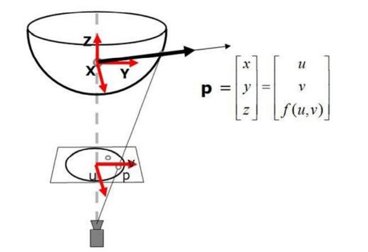
投影结构也是类似的形式：通过一个球面投影到归一化平面上。

其中
f ρ = a 0 + a 1 ρ 2 + a 2 ρ 3 + a 4 ρ 4 + … ρ = u 2 + v 2 \begin{gathered} f_{\rho}=a_{0}+a_{1} \rho^{2}+a_{2} \rho^{3}+a_{4} \rho^{4}+\ldots \\ \rho=\sqrt{u^{2}+v^{2}} \end{gathered} fρ​=a0​+a1​ρ2+a2​ρ3+a4​ρ4+…ρ=u2+v2 ​​
上述我们使用模型将图像平面和 3D 点进行了关联，考虑到实际像素平面可以近似使用一个仿射变换来得到, 于是有
[ u ′ v ′ ] = [ c d e 1 ] [ u v ] + [ x c ′ y c ′ ] \left[\begin{array}{l} u^{\prime} \\ v^{\prime} \end{array}\right]=\left[\begin{array}{ll} c & d \\ e & 1 \end{array}\right]\left[\begin{array}{l} u \\ v \end{array}\right]+\left[\begin{array}{l} x_{c}^{\prime} \\ y_{c}^{\prime} \end{array}\right] [u′v′​]=[ce​d1​][uv​]+[xc′​yc′​​]
可以看到, 其实这个模型从像素坐标到世界坐标系时非常简单，只要按照多项式计算即可。相反，其从世界坐标系到相机 坐标系投影会更加麻烦。

• 这个是matlab代码
• 正向投影：

%WORLD2CAM projects a 3D point on to the image
%   m=WORLD2CAM(M, ocam_model) projects a 3D point on to the
%   image and returns the pixel coordinates.
%   
%   M is a 3xN matrix containing the coordinates of the 3D points: M=[X;Y;Z]
%   "ocam_model" contains the model of the calibrated camera.
%   m=[rows;cols] is a 2xN matrix containing the returned rows and columns of the points after being
%   reproject onto the image.
%   
%   Copyright (C) 2006 DAVIDE SCARAMUZZA   
%   Author: Davide Scaramuzza - email: davide.scaramuzza@ieee.org

function m=world2cam(M, ocam_model)  %M：3d点
ss = ocam_model.ss;    %
xc = ocam_model.xc;
yc = ocam_model.yc;
width = ocam_model.width;
height = ocam_model.height;
c = ocam_model.c; %对应模型的c，d，e
d = ocam_model.d;
e = ocam_model.e;

[x,y]  = omni3d2pixel(ss,M,width, height); % p = [x,y,z]^T = [u,v,f(u,v)]
m(1,:) = x*c + y*d + xc;
m(2,:) = x*e + y   + yc;

function [x,y] = omni3d2pixel(ss, xx, width, height)


%convert 3D coordinates vector into 2D pixel coordinates

%These three lines overcome problem when xx = [0,0,+-1]
ind0 = find((xx(1,:)==0 & xx(2,:)==0));
xx(1,ind0) = eps;
xx(2,ind0) = eps;

m = xx(3,:)./sqrt(xx(1,:).^2+xx(2,:).^2); % 把第三项做了归一化 z = z/sqrt(x^2+y^2)

rho=[];
poly_coef = ss(end:-1:1);
poly_coef_tmp = poly_coef;
for j = 1:length(m)
    poly_coef_tmp(end-1) = poly_coef(end-1)-m(j); % 把多项式中的a0-m 让z = g(m) 也就是z=多项式
    											  % a0+a1ρ^2+a2ρ^3+a4ρ^4 = m
    rhoTmp = roots(poly_coef_tmp);
    res = rhoTmp(find(imag(rhoTmp)==0 & rhoTmp>0));% & rhoTmp<height ));    %obrand
    if isempty(res) %| length(res)>1    %obrand
        rho(j) = NaN;
    elseif length(res)>1    %obrand
        rho(j) = min(res);    %obrand
    else
        rho(j) = res;
    end
end
x = xx(1,:)./sqrt(xx(1,:).^2+xx(2,:).^2).*rho ;
y = xx(2,:)./sqrt(xx(1,:).^2+xx(2,:).^2).*rho ;

• 反向投影

对应到原理 [ u ′ v ′ ] = [ c d e 1 ] [ u v ] + [ x c ′ y c ′ ] \left[\begin{array}{l} u^{\prime} \\ v^{\prime} \end{array}\right]=\left[\begin{array}{ll} c & d \\ e & 1 \end{array}\right]\left[\begin{array}{l} u \\ v \end{array}\right]+\left[\begin{array}{l} x_{c}^{\prime} \\ y_{c}^{\prime} \end{array}\right] [u′v′​]=[ce​d1​][uv​]+[xc′​yc′​​]就是已知 [ u ′ v ′ ] \left[\begin{array}{l} u^{\prime} \\ v^{\prime} \end{array}\right] [u′v′​]求 [ u v ] \left[\begin{array}{l} u \\ v \end{array}\right] [uv​]

%CAM2WORLD Project a give pixel point onto the unit sphere
%   M=CAM2WORLD=(m, ocam_model) returns the 3D coordinates of the vector
%   emanating from the single effective viewpoint on the unit sphere
%
%   m=[rows;cols] is a 2xN matrix containing the pixel coordinates of the image
%   points.
%
%   "ocam_model" contains the model of the calibrated camera.
%   
%   M=[X;Y;Z] is a 3xN matrix with the coordinates on the unit sphere:
%   thus, X^2 + Y^2 + Z^2 = 1
%   
%   Last update May 2009
%   Copyright (C) 2006 DAVIDE SCARAMUZZA   
%   Author: Davide Scaramuzza - email: davide.scaramuzza@ieee.org

function M=cam2world(m, ocam_model)

n_points = size(m,2);

ss = ocam_model.ss;
xc = ocam_model.xc;
yc = ocam_model.yc;
width = ocam_model.width;
height = ocam_model.height;
c = ocam_model.c;
d = ocam_model.d;
e = ocam_model.e;

A = [c,d;
     e,1];
T = [xc;yc]*ones(1,n_points);

m = A^-1*(m-T); % 相当于[c,d,e,1]^T*([u',v']-[xc',yc'])
M = getpoint(ss,m);
M = normc(M); %normalizes coordinates so that they have unit length (projection onto the unit sphere)

function w=getpoint(ss,m)

% Given an image point it returns the 3D coordinates of its correspondent optical
% ray

w = [m(1,:) ; m(2,:) ; polyval(ss(end:-1:1),sqrt(m(1,:).^2+m(2,:).^2)) ]; % [u,v,多项式]

畸变模型

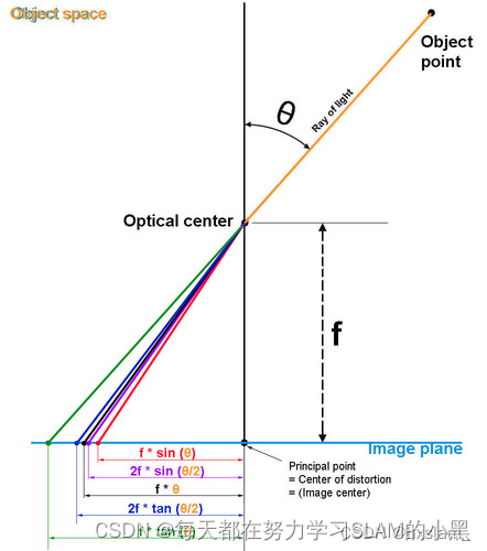
1. Equidistant (EQUI) 等距畸变模型

Equidistant 有四个参数： [ k 1 , k 2 , k 3 , k 4 ] [k_1,k_2,k_3,k_4] [k1​,k2​,k3​,k4​]

P s = P ∥ P ∥ = ( x s , y s , z s ) r = ( x s 2 + y s 2 ) θ = a t a n 2 ( r , ∣ z s ∣ ) = a t a n 2 ( r , 1 ) = a t a n ( r ) θ d = θ ( 1 + k 1 θ 2 + k 2 θ 4 + k 3 θ 6 + k 4 θ 8 ) P_{s}=\frac{P}{\|P\|}=\left(x_{s}, y_{s}, z_{s}\right)\\ r = \sqrt{(x_s^2+y_s^2)} \\ \theta = atan2(r,|z_s|) = atan2(r,1) = atan(r) \\ \theta_d =\theta(1+k_1\theta^2+k_2\theta^4+k_3\theta^6+k_4\theta^8)\\ Ps​=∥P∥P​=(xs​,ys​,zs​)r=(xs2​+ys2​) ​θ=atan2(r,∣zs​∣)=atan2(r,1)=atan(r)θd​=θ(1+k1​θ2+k2​θ4+k3​θ6+k4​θ8)

{ x d = θ d x s r y d = θ d y s r \left\{ \begin{matrix} x_d = \frac{\theta_dx_s}{r}\\ y_d = \frac{\theta_dy_s}{r} \end{matrix} \right. { xd​=rθd​xs​​yd​=rθd​ys​​​

float ix = (x - ocx) / ofx;
float iy = (y - ocy) / ofy;
float r = sqrt(ix * ix + iy * iy);
float theta = atan(r);
float theta2 = theta * theta;
float theta4 = theta2 * theta2;
float theta6 = theta4 * theta2;
float theta8 = theta4 * theta4;
float thetad = theta * (1 + k1 * theta2 + k2 * theta4 + k3 * theta6 + k4 * theta8);
float scaling = (r > 1e-8) ? thetad / r : 1.0;
float ox = fx*ix*scaling + cx;
float oy = fy*iy*scaling + cy;

2. Radtan 切向径向畸变， Brown模型

Radtan有四个参数： [ k 1 , k 2 , p 1 , p 2 ] [k_1,k_2,p_1,p_2] [k1​,k2​,p1​,p2​]

{ x d i s t o r t e d = x ( 1 + k 1 r 2 + k 2 r 4 ) + 2 p 1 x y + p 2 ( r 2 + 2 x 2 ) y d i s t o r t e d = y ( 1 + k 1 r 2 + k 2 r 4 ) + 2 p 2 x y + p 1 ( r 2 + 2 y 2 ) \left\{ \begin{matrix} x_{distorted} = x(1+k_1r^2+k_2r^4)+2p_1xy+p_2(r^2+2x^2)\\ y_{distorted} = y(1+k_1r^2+k_2r^4)+2p_2xy+p_1(r^2+2y^2) \end{matrix} \right. { xdistorted​=x(1+k1​r2+k2​r4)+2p1​xy+p2​(r2+2x2)ydistorted​=y(1+k1​r2+k2​r4)+2p2​xy+p1​(r2+2y2)​
其中x,y是不带畸变的坐标, x d i s t o r t e d , y d i s t o r t e d x_{distorted},y_{distorted} xdistorted​,ydistorted​​是有畸变图像的坐标。

// cam2world(distorted2undistorted)
// 先经过内参变换，再进行畸变矫正
{
  
  cv::Point2f uv(u,v), px;
  const cv::Mat src_pt(1, 1, CV_32FC2, &uv.x);
  cv::Mat dst_pt(1, 1, CV_32FC2, &px.x);
  cv::undistortPoints(src_pt, dst_pt, cvK_, cvD_);
  xyz[0] = px.x;
  xyz[1] = px.y;
  xyz[2] = 1.0;
}
// 先经过镜头发生畸变，再成像过程，乘以内参
// world2cam(undistorted2distorted)
{
  
  double x, y, r2, r4, r6, a1, a2, a3, cdist, xd, yd;
  x = uv[0];
  y = uv[1];
  r2 = x*x + y*y;
  r4 = r2*r2;
  r6 = r4*r2;
  a1 = 2*x*y;
  a2 = r2 + 2*x*x;
  a3 = r2 + 2*y*y;
  cdist = 1 + d_[0]*r2 + d_[1]*r4 + d_[4]*r6;
  xd = x*cdist + d_[2]*a1 + d_[3]*a2;
  yd = y*cdist + d_[2]*a3 + d_[3]*a1;
  px[0] = xd*fx_ + cx_;
  px[1] = yd*fy_ + cy_;
}

3. FOV 视野畸变模型

FOV 有一个参数： [ ω ] [\omega] [ω]

P s = P ∥ P ∥ = ( x s , y s , z s ) r = ( X / Z ) 2 + ( Y / Z ) 2 = x 2 + y 2 r d = 1 ω a r c t a n ( 2 ⋅ r ⋅ t a n ( ω / 2 ) ) P_{s}=\frac{P}{\|P\|}=\left(x_{s}, y_{s}, z_{s}\right)\\ r = \sqrt{(X/Z)^2 + (Y/Z)^2} = \sqrt{x^2+y^2}\\ r_d = \frac{1}{\omega}arctan(2\cdot r \cdot tan(\omega /2)) Ps​=∥P∥P​=(xs​,ys​,zs​)r=(X/Z)2+(Y/Z)2 ​=x2+y2 ​rd​=ω1​arctan(2⋅r⋅tan(ω/2))

{ x d i s t o r t e d = r d r ⋅ x s y d i s t o r t e d = r d r ⋅ y s \left\{ \begin{matrix} x_{distorted} = \frac{r_d}{r}\cdot x_s\\ y_{distorted} = \frac{r_d}{r}\cdot y_s \end{matrix} \right. { xdistorted​=rrd​​⋅xs​ydistorted​=rrd​​⋅ys​​

// cam2world(distorted2undistorted)
Vector2d dist_cam( (x - cx_) * fx_inv_, (y - cy_) * fy_inv_ );
double dist_r = dist_cam.norm();
double r = invrtrans(dist_r);
double d_factor;
if(dist_r > 0.01)
  d_factor =  r / dist_r;
else
  d_factor = 1.0;
return unproject2d(d_factor * dist_cam).normalized();


// world2cam(undistorted2distorted)
double r = uv.norm();
double factor = rtrans_factor(r);
Vector2d dist_cam = factor * uv;
return Vector2d(cx_ + fx_ * dist_cam[0],
                  cy_ + fy_ * dist_cam[1]);

// 函数
//! Radial distortion transformation factor: returns ration of distorted / undistorted radius.
inline double rtrans_factor(double r) const
{
  
  if(r < 0.001 || s_ == 0.0)
    return 1.0;
  else
    return (s_inv_* atan(r * tans_) / r);
};

//! Inverse radial distortion: returns un-distorted radius from distorted.
inline double invrtrans(double r) const
{
  
  if(s_ == 0.0)
    return r;
  return (tan(r * s_) * tans_inv_);
};

投影模型

1. 全投影模型

1. 将世界系下的世界坐标系点投影到归一化球面上（unit sphere）
( X ) F m → ( X s ) F m = X ∥ X ∥ = ( X s , Y s , Z s ) (\mathcal{X})_{\mathcal{F}_{m}} \rightarrow\left(\mathcal{X}_{s}\right)_{\mathcal{F}_{m}}=\frac{\mathcal{X}}{\|\mathcal{X}\|}=\left(X_{s}, Y_{s}, Z_{s}\right) (X)Fm​​→(Xs​)Fm​​=∥X∥X​=(Xs​,Ys​,Zs​)
2. 将投影点的坐标变换到一个新坐标系下表示, 新坐标系的原点位于 C p = ( 0 , 0 , ξ ) \mathcal{C}_{p}=(0,0, \xi) Cp​=(0,0,ξ)
( X s ) F m → ( X s ) F p = ( X s , Y s , Z s + ξ ) \left(\mathcal{X}_{s}\right)_{\mathcal{F}_{m}} \rightarrow\left(\mathcal{X}_{s}\right)_{\mathcal{F}_{p}}=\left(X_{s}, Y_{s}, Z_{s}+\xi\right) (Xs​)Fm​​→(Xs​)Fp​​=(Xs​,Ys​,Zs​+ξ)
3. 将其投影到归一化平面 ( m u \mathbf{m}_{u} mu​归一化坐标点）
m u = ( X s Z s + ξ , Y s Z s + ξ , 1 ) = ℏ ( X s ) \mathbf{m}_{u}=\left(\frac{X_{s}}{Z_{s}+\xi}, \frac{Y_{s}}{Z_{s}+\xi}, 1\right)=\hbar\left(\mathcal{X}_{s}\right) mu​=(Zs​+ξXs​​,Zs​+ξYs​​,1)=ℏ(Xs​)
4. 增加畸变影响
m d = m u + D ( m u , V ) \mathbf{m}_{d}=\mathbf{m}_{u}+D\left(\mathbf{m}_{u}, V\right) md​=mu​+D(mu​,V)
5. 乘上相机模型内参矩阵 K \mathbf{K} K, 其中 γ \gamma γ 表示焦距, ( u 0 , v 0 ) \left(u_{0}, v_{0}\right) (u0​,v0​) 表示光心, s s s 表示坐标系倾斜系数, r r r 表示纵横比
p = K m = [ γ γ s u 0 0 γ r v 0 0 0 1 ] m = k ( m ) \mathbf{p}=\mathbf{K m}=\left[\begin{array}{ccc} \gamma & \gamma s & u_{0} \\ 0 & \gamma r & v_{0} \\ 0 & 0 & 1 \end{array}\right] \mathbf{m}=k(\mathbf{m}) p=Km=⎣⎡​γ00​γsγr0​u0​v0​1​⎦⎤​m=k(m)

常用模型组合

MEI Camera： Omni + Radtan

Pinhole Camera：Pinhole + Radtan

atan Camera: Pinhole + FOV

Davide Scaramuzza Camera

这个是ETHZ的工作，畸变和相机内参放在一起了，为了克服针对鱼眼相机参数模型的知识缺乏，使用一个多项式来代替

DSO：Pinhole + Equi / Radtan / FOV
VINS：Pinhole / Omni + Radtan
SVO：Pinhole / atan / Scaramuzza
OpenCV：cv: pinhole + Radtan , cv::fisheye: pinhole + Equi , cv::omnidir: Omni + Radtan